| Articles | ||||||||||||||||||
|
Shallow−Water Acoustics Extracting a signal from noise can be complicated, especially along a coastline filled with marine life, shipping lanes, undersea waves, shelves, and fronts that scatter sound. During the two world wars, oceanographers studied both shallowand deep−water acoustics. But during the cold war, the research emphasis shifted abruptly to deep water, where the ballistic missile submarine threat lurked (see box 1). After the cold war, the onset of regional conflicts in coastal countries shifted the focus again to shallow water. Those waters encompass about 5% of the world's oceans on the continental shelves, roughly the region from the beach to the shelf break, where water depths are about 200 meters. To a significant extent, the problems of shallow−water acoustics are the same as those encountered in nondestructive testing, medical ultrasonics, multichannel communications, seismic processing, adaptive optics, and radio astronomy. In these fields, propagating waves carry information, embedded within some sort of noise, to the boundaries of a minimally accessible, poorly known, complex medium, where it is detected.1,2 Although submarine detection has driven much of the acoustics research, other important applications have emerged, such as undersea communications, mapping of the ocean's structure and topography, locating mines or archaeological artifacts, and the study of ocean biology. Shallow water is usually a noisy environment because shipping lanes exist along coastlines. Submarines typically radiate in the same frequency band as shipping noise, less than 1 kilohertz. The proliferation of quiet submarine technology has restimulated the development of active sonar systems, which send out pulses and examine their echoes, rather than the more stealthy, passive approach of listening and exploiting the relevant physics. However, the ultimate limits of passive acoustics in terms of signal−to−noise ratio (SNR), acoustic aperture (or antenna) size, and the ocean environment are ongoing research issues. The sound speed in water is about 1500 m/s, so wavelengths of interest are on the order of a few meters. In shallow water, with boundaries framed by the surface and bottom, the typical depth−to−wavelength ratio is about 10−100. That ratio makes the propagation of acoustic waves there analogous to electromagnetic propagation in a dielectric waveguide. But the shallow ocean is an exceedingly complicated place. The surface and the ocean's index of refraction have a spatial and time dependence, and the presence of ocean inhomogeneities and loud ships can frequently scatter, jam, or mask the most interesting sounds. So, whether using active or passive techniques, scientists are ultimately concerned with the physics of extracting a signal that propagates in a lossy, dynamic waveguide from noise influenced by that same waveguide's complexity. In that light, and considering our still imperfect understanding of coastal oceanography, one can begin to appreciate shallow−water acoustics as an interdisciplinary blend of physics, signal processing, physical oceanography, marine geophysics, and even marine biology. Ocean waveguides
Because the motions of ocean waves and water masses, along with the sources and receivers of signals that pass through them, are so small compared to the speed of sound in seawater, the ocean, to first approximation, can be treated as essentially a frozen medium. One can further model the ocean and seabed as horizontally stratified, a simplification that permits the basic waveguide description of signal propagation there. The vertical variation in the layering is typically much greater than the horizontal variation, a fact that minimizes out−of−plane refraction, diffraction, and scattering (with some notable exceptions). Moreover, temperature, T (in Celsius), provides an excellent characterization of sound speed, c, because the depth plays a minor role in shallow water: c ≈ 1449 + 4.6T + (1.34 − 0.01T)(S − 35) + 0.016z, where the depth z is in meters, S is salinity in parts per thousand, and the last term embodies density and static pressure effects. The seabed can often be approximated as a fluid medium, with only sound speed, attenuation, and density as acoustic variables.
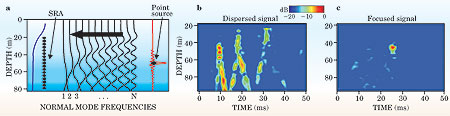
Box 2 summarizes the solution to the wave equation for the canonical shallow−water acoustic waveguide. To appreciate its application to a realistic case, consider the panels in figure 2, which show the behavior of a sound wave excited by a point source in a waveguide. The propagating normal modes have different frequency−dependent group speeds, so a finite−bandwidth pulse disperses as it propagates down the waveguide and passes an array of detectors. The lower modes become trapped toward the bottom of the waveguide because sound paths bend toward regions of lower sound speeds. The lowest mode has the most direct path down the waveguide and arrives at the detectors first. Higher modes follow and refract higher in the water column's thermocline.
To send and receive
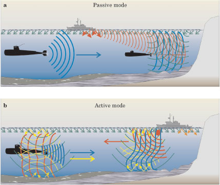
The lower panel illustrates the case of active sonar, which transmits pulses and extracts information from their echoes. Monostatic sonar locates the transmitter and receiver together, as pictured; in bistatic sonar, those pieces are remote from each other. In addition to ASW, active sonars are useful in, for example, communications, mine hunting, archaeological research, imaging of ocean and seabed features, and finding fish. One non−ASW application is to image internal−wave fields in the ocean using sound scattered from zooplankton that drift with the water. Based on the Doppler shift of the returned echo, the water velocity can be mapped as a function of its position. Currently, plane−wave beamforming4 is the workhorse of both types of sonar. Just as in electromagnetics, a phased array of antennas directs a signal to interfere constructively in a particular "look" direction. To resolve as much information from the signal as possible, researchers have also created synthetic apertures.5 The idea is to send a series of brief pulses from a ship that moves through some distance in time, and then, based on the signals sent and received, construct a large, high−resolution aperture. In active sonar systems, this method is allowing oceanographers to accurately map the ocean floor. Passive synthetic aperture sonar is more challenging: Source frequencies are typically unknown, and the spacefrequency ambiguity affects the performance of the aperture. Moreover, even the ability to construct a synthetic aperture is not assured. It depends strongly on the temporal coherence of the source and the coherence properties of the acoustic field itself related to the complexity of a dynamic ocean. The dynamic ocean
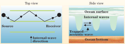
Dynamical phenomena in the ocean introduce challenges beyond those encountered when acoustic fields propagate through a complex but static medium. The presence of internal waves (see box 3) and coastal fronts, for example, adds frequencyand time−dependent complexity to acoustic propagation in shallow water. The nearly ubiquitous linear internal waves provide a continuous scattering mechanism for redistributing acoustic energy in the oceans. In contrast, nonlinear internal waves, such as solitons, provide strong, discrete scattering events6 due to their generally higher amplitude and shorter wavelength. Because nonlinear internal waves are more directional than the random, isotropic linear internal waves, they can produce a strong azimuthal dependence in the scattering. Some interesting phenomena can occur when an acoustic signal encounters a nonlinear wave. When the signal path happens to run parallel to the propagation direction of the nonlinear internal waves (perpendicular to the internal wave wavefronts), for instance, the acoustic normal modes (with wavenumbers kn, km, . . .) couple strongly, particularly when there is a Bragg resonance condition, given by D = 2π/(kn − km), between the internal soliton spacing D and the spatial interference distance between two modes. Jixun Zhou and Peter Rogers of Georgia Tech, working with scientists from China, first observed such effects in the Yellow Sea.7 The mode coupling produced strong frequency−dependent nulls in the acoustic field; those nulls differed by as much as 40 dB between scattering and nonscattering conditions. Signal amplification has shown up in other experiments due to the same scattering mechanism.
Coastal fronts in shallow water interact similarly with sound. A sound wave that propagates directly across an ocean thermal front encounters a sharp sound−speed gradient, and strong mode coupling occurs. For acoustic propagation at small grazing angles to the front, the effect produces total internal reflection. Signal processing
Here we discuss recent research efforts to extract signals from noise while coping with, and even exploiting, the waveguide properties of the shallow−water environment. A large aperture, that is, a detector array filled with many elements, provides high resolution or focusing capability because of the wavenumber (or angle) spread that it can efficiently sample. Complexity can be thought of as the wavenumber diversity in a waveguide or scattering medium. Paradoxically, it's possible to focus an acoustic signal more accurately when that signal travels through a complicated medium than when it doesn't. Various research groups have combined multisensor apertures with a complex medium to enhance signal processing in areas such as communications, medical ultrasonics, seismology, and matched−field acoustics.1
An alternative to performing this model−based processing is to use phase conjugation (PC) or its Fourier transform, time reversal (TR), to reconstruct the original waveform after it has passed through a noisy medium. Typically, one takes the complex conjugated or time−reversed data from a signal that strikes a detector array to be the source excitations that are retransmitted through the same medium (figure 2c). The PC/TR process is then equivalent to correlating the measured data with a transfer function from the array to locate the original source. Both MFP and PC are thus signal−processing analogs to the guide−star and mechanical−lens−adjustment feedback technique used in adaptive optics:8 MFP uses data together with a model to fine−tune that model, whereas PC/TR is an active form of adaptive optics. PC/TR requires large transmission arrays to do the job. Currently, that technique serves only as an ocean acoustic tool to help researchers understand the ocean's capacity to support coherent wave information in an assortment of complicated environments. Future directions
Acoustics. The complicated nature of the oceanits uneven bottom, internal waves, solitons and fronts, and source and receiver motion, for examplerequires signal−processing methods that can account for motion and medium uncertainty. The same problem exists in fields such as medical ultrasonic imaging, for which placing the focus of an object in a complex, moving region is essential. But most signal−processing research has emphasized free−space propagation in static or near−static conditions. And theoreticians have not adequately developed a foundation for using dynamic complexity to enhance the processing results. The challenge is to develop methods that use the data themselves and the physics of signal propagation through complex media as the mainstays of adaptive processing or inversion methods to determine medium properties. This approach is particularly appropriate in shallow water, because the ocean modulates the complexity of the acoustic field that interacts with an inhomogeneous, porous, and elastic ocean bottom. Adaptive processing algorithms use the data to construct a modified (plane−wave or waveguide) replica vector to enhance resolution and minimize sidelobes, the (ordinarily) small peaks found in beamforming. When evaluating a candidate position, the so−called minimum variance distortionless processor minimizes or nulls contributions from other positions.3,5 The nulling out of interferers, such as loud ships on the surface, is important because their sounds coming through the sidelobes are typically louder than the signals of interest. Adaptive processors are, however, very sensitive to data sample size, noise, dynamics, and mismatch between replicas and the actual ocean acoustic environment. Because of the sensitivity, it is critical to accurately model features such as the complex ocean bottom. The complexity of the bottom interaction is of special interest in very shallow regions (tens of meters or less), in which acoustic detection of mines from a safe distance is important. Shallow−water noise and reverberation, conventionally thought to be nuisances, are now becoming useful information as new inversion methods are being developed.9 High−frequency acoustics is another, albeit unexpected, emerging research topic10; based on deep−water acoustics, researchers had previously thought that ray solutions in the high−frequency regime were adequate. Active sonar. Signal design poses an interesting challenge. A Heisenberg uncertainty relation that exists between range and Doppler (velocity) resolution is further complicated by the presence of a time−varying, reverberant channel. The research problem is to design signals that use various modulation schemes for a specific sonar task, such as determining position and motion or coherently communicating information.11 Research is just beginning in the field of multichannel (multiple−input multiple−output, or MIMO) undersea communications, in which the total information capacity of the channel is a fundamental issue. Multiple signals are sent between multiantenna arrays (see the article by Steve Simon, Aris Moustakas, Marin Stoytchev, and Hugo Safar in Physics Today, September 2001, page 38). Similarly, dealing with resonances in, or even below, a waveguide when sound scatters from elastic targets poses theoretical and measurement challenges. Dynamics and signal processing. In shallow water, to cancel out noise from a loud, moving surface ship requires dealing with its motion using resolution cells over the time it takes to construct a data correlation matrix. That time may be from seconds to minutes, a delay that can confuse the cancellation process.12 Consequently, very high resolution can sometimes be bad for a system. On the other hand, there exists a transition range beyond which resolution cells are large enough to accommodate source motion, but the dynamic ocean still blurs the signal. One way to deal with blurringat least in mild casesis to create an ensemble of replica vectors from our knowledge of the ocean dynamics.13 For more extreme oceanographic distortion, nonlinear optimization methods, such as simulated annealing or genetic algorithms, might be relevant and extendable to practical cases.14 Another potential advantage of such methods is their flexibility: Data from diverse sensors such as satellite measurements of sea conditions can be integrated. Finally, the emerging development and use of unmanned underwater vehicles (UUVs) provide new opportunities and challenges for almost all the topics in shallow−water acoustics mentioned in this article. Clearly, the research challenges of shallow−water acoustics exist in many other fields; complexity is not limited to ocean phenomena. The hope, therefore, is that the wave propagation and signal−processing advances that ocean acousticians are making will find applications in other fields, and vice versa. We greatly appreciate assistance from Tuncay Akal, Aaron Thode, Philippe Roux, Hee Chun Song, Rob Pinkel, Katherine Kim, Art Newhall, and Harry Cox. The Office of Naval Research supported much of the research discussed in this article. Some of that research was performed in collaboration with the NATO Undersea Research Center in La Spezia, Italy.
1. M. Fink, W. A. Kuperman, J. P. Montagner, A.
Tourin, eds., Imaging of Complex Media With Acoustic and Seismic
Waves, Springer, New York (2002).
2. L. M. Brekhovskikh, Yu P. Lysanov, Fundamentals
of Ocean Acoustics, 2nd ed., Springer-Verlag, New York (1991);
F. B. Jensen. W. A. Kuperman, M. B. Porter, H. Schmidt,
Computational Ocean Acoustics, AIP Press, Springer, New York
(2000); B. Katsnelson, V. Petnikov, Shallow Water Acoustics,
Springer, New York (2002); W. A. Kuperman, G. L. D'Spain, eds.,
Ocean Acoustic Interference Phenomena and Signal Processing,
AIP, Melville, NY (2002); H. Medwin, C. S. Clay, Fundamentals of
Acoustic Oceanography, Academic Press, Boston, MA (1998).
3. A. B. Baggeroer, W. A. Kuperman, P. N.
Mikhalevsky, IEEE
J. Ocean. Eng. 18, 401 (1993) [INSPEC].
4. D. H. Johnson, D. E. Dudgeon, Array Signal
Processing: Concepts and Techniques, Prentice Hall, Englewood
Cliffs, NJ (1993).
5. R. J. Urick, Principles of Underwater
Sound, 3rd ed., McGraw-Hill, New York (1983). See also the
special issue on synthetic aperture sonar, IEEE J. Ocean. Eng.
17 (1992).
6. M. Badiey, J. Lynch, X. Tang, J. Apel, SWARM
Group, IEEE J.
Ocean. Eng. 27, 117 (2002) [INSPEC].
7. J. X. Zhou, X. S. Zhang, P. J. Rogers, J.
Acoust. Soc. Am. 90, 2042 (1991) [INSPEC].
8. M. Siderius, D. R. Jackson, D. Rouseff, R. Porter,
J. Acoust.
Soc. Am. 102, 3439 (1997) [INSPEC].
9. M. J. Buckingham, B. V. Berkhouse, S. A. L. Glegg,
Nature
365, 327 (1992) [INSPEC];
C. H. Harrison, J. Acoust. Soc.
Am. 115, 1505 (2004) [SPIN];
for reverberation inversion and related subjects, see the special
issue on ocean acoustic inversion, IEEE J. Ocean. Eng.
29 (2004).
10. M. B. Porter, M. Siderius, W. A. Kuperman, eds.,
High-Frequency Ocean Acoustics, AIP Press, Melville, NY
(2004).
11. D. B. Kilfoyle, A. B. Baggeroer, IEEE J. Ocean. Eng.
25, 4 (2000) [INSPEC].
12. Moving interferers and adaptive processing in
shallow water were first discussed in A. B. Baggeroer, H. Cox,
Proc. 33rd Asilomar Conference on Signals, Systems and
Computers, M. B. Matthews, ed., IEEE Computer Society, Pacific
Grove, CA (1999), and H. Cox, Proc. 2000 IEEE Sensor Array and
Multichannel Signal Processing Workshop, S. Smith, ed., IEEE,
Cambridge, MA (2000). See also H. C. Song, W. A. Kuperman, W. S.
Hodgkiss, P. Gerstoft, J. S. Kim, IEEE J. Ocean. Eng.
28, 250 (2003).
13. J. L. Krolik, J. Acoust. Soc. Am.
92, 1402 (1992).
14. M. D. Collins, W. A. Kuperman, J. Acoust. Soc.
Am. 90, 1410 (1991) [INSPEC];
P. Gerstoft, J. Acoust. Soc. Am. 95, 770
(1994) [INSPEC];
A. M. Thode, G. L. D'Spain, W. A. Kuperman, J. Acoust. Soc.
Am. 107, 1286 (2000) [INSPEC];
S. E. Dosso, Inverse
Probl. 19, 419 (2003) .
15. S. Kim et al., J. Acoust. Soc.
Am. 114, 145 (2003) [SPIN].
16. N. O. Booth et al., IEEE J. Ocean. Eng.
21, 402 (1996) [INSPEC].
17. S. Pond, G. L. Pickard, Introductory Dynamic
Oceanography, Pergamon Press, New York (1978).
18. B. J. Sperry, J. F. Lynch, G. Gawarkiewicz, C. S.
Chiu, A. Newhall, IEEE J. Ocean. Eng. 28, 729
(2003).
Bill Kuperman is a
professor at the Scripps Institution of Oceanography of the
University of California, San Diego. Jim Lynch is a
senior scientist at the Woods Hole Oceanographic Institution in
Woods Hole, Massachusetts.
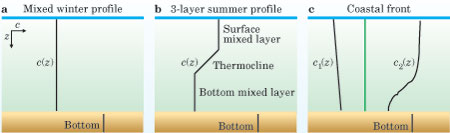
Figure 1. Three models of the speed of sound c(z) in seawater encompass a wide variety of shallow−water oceanography. (a) An ocean with a constant sound speed represents fully mixed temperature conditions found during the winter in Earth's mid latitudes and in water shallower than about 30 meters. (b) The common three−layer model consists of two separate mixed layers, both of constant temperature and sound speed, with a thermocline gradient sandwiched in between. (c) In a coastal front model, two water masses with differing temperature profiles meet at a vertical wall (green). Note that the ocean bottom has a higher sound speed and density, indicated by its shift to the right, than the water layer.
Box 1. Ocean Acoustics During the Cold War
The speed of sound in the ocean decreases as the water cools but increases with depth. In 1943, Maurice Ewing and Joe Worzel discovered the deep sound channel (DSC), an acoustic waveguide that forms by virtue of a minimum in that temperature−dependent sound speed. That minimum (plotted below as a dotted line) typically follows a path that varies from the cold surface at the poles to a depth of about 1300 meters at the equator. Because sound refracts toward lower sound speeds, ocean noises that enter the DSC oscillate about the sound−speed minimum and can propagate thousands of kilometers. 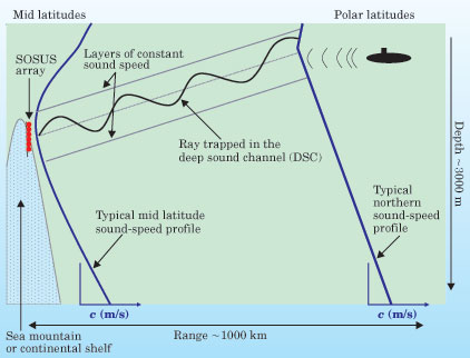 In the 1950s, the US Navy exploited that property when it created the multibillion−dollar SOSUS (Sound Ocean Surveillance System) network to monitor Soviet ballistic−missile nuclear submarines. The network consisted of acoustic antennas placed on ocean mountains or continental rises whose height extended into the DSC. Those antennas were hardwired to land stations using undersea telephone cables. Submarines typically go down to depths of a few hundred meters, and during the cold war, many were loitering in polar waters, where their telltale noises coupled to the shallower regions of the DSC. Those noises usually came from poorly machined parts, such as the propeller. Used successfully for many decades, SOSUS became, in effect, a major cold war victory. The system was eventually compromised by the Walker spy episode, which prompted the Soviets to introduce better−machined components and hence build a quieter fleet of submarines. Nowadays, the basic antisubmarine warfare challenge is to detect quiet diesel−electric submarines in noisy, coastal waters.
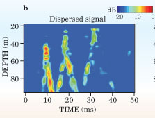
Figure 2. Shallow−water waveguide. (a) A point source launches a 2−millisecond acoustic pulse that excites a series of normal modes that propagate in an ocean with a summer sound−speed profile (the purple line). The lower modes are trapped below the thermocline. (b) Because of modal dispersion, the signal arrives at the source−receiver array (SRA)8 km from where it startedwith more than a 40 ms spread. (c) Time reversal of the pulse at the SRA (retransmitting the last arrival first, and so on, back through the waveguide) produces a recompressed focus at the original point source position. The pulse's focal size is commensurate with the shortest wavelength of the highest surviving mode. (Adapted from ref. 15.)
Box 2. Normal Modes in Shallow Water
The canonical (Pekeris) shallow−water acoustic waveguide2 has a constant sound speed, mirror reflection at the surface, and a grazing−angle−dependent reflectivity at the ocean bottom. The classic plane−wave Rayleigh−reflection coefficient, used to describe electromagnetic waves at a dielectric interface, can similarly describe reflection from the bottom interface. That interface has a critical angle θctypically about 15°, depending on the material there. As shown in the upper panel of the figure, a source in such a waveguide produces a sound field that propagates at angles confined to a cone of 2θc. Within that cone, constructive interference selects discrete propagation angles; outside the cone, waves disappear into the bottom after a few reflections. Separation of variablesrange and depth, assuming azimuthal symmetry about zproduces solutions to the Helmholtz equation, which describes waveguide propagation. The depth equation is an eigenvalue problem that yields a set of normal modes satisfying the preceding boundary conditions. When combined with the range solution, the modes propagate along the waveguide and spread cylindrically. The pressure field from a point source located at a particular range and depth (0,zs) is given by the normal−mode sum solution to the Helmholtz equation (for r >> l), 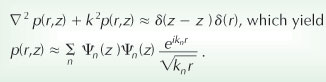 In the solution, k = ω/c, where ω is angular frequency and c the sound speed. The normal modes Ψn(z) and horizontal wavenumbers kn are obtained from the eigenvalue problem. The normal modes of the Pekeris waveguide, shown in the figure's bottom panel, are sine waves that vanish at the surface and abruptly change to decaying exponentials at the bottom boundary. Because they are evanescent (or nonpropagating) there, the modes are "trapped" in the water column. The attenuation of sound in the bottom is the major loss mechanism in shallow water and is proportional to the shaded area of the decaying mode. For a simple sinusoid, each modal term in the pressure sum describes propagating waves with wavenumber magnitude k and angles to the horizontal given by cos θn = kn/k within the critical angle cone cos−1(kn/k) < θc. Each mode has its own phase and group speed. 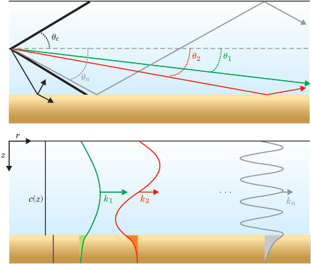
Figure 3. Sonar detection. (a) In this passive sonar scheme, the submarine on the right uses a towed array of detectors to distinguish sounds that originate from the one to the left. The towed array provides a large aperture to discriminate the desired signal (blue) that is distorted by the shallow−water environment and embedded in ocean surface noise (green) and shipping noise (red). (b) In active sonar, the ship sends out a pulse (red). Its echo (blue), distorted by the shallow−water environment, returns to the ship's receiver, which tries to distinguish it from backscattered reverberation (yellow) and ocean noise (green).
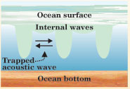
Figure 4. Geometry for the ducting of sound between nonlinear internal waves. The internal waves produce alternating highand low−temperature (and thus sound−speed) regions in the water as they move through the ocean. Snell's law pushes the sound toward the low−speed region (blue) between the high−speed internal−wave wavefronts (green), thus confining it there.
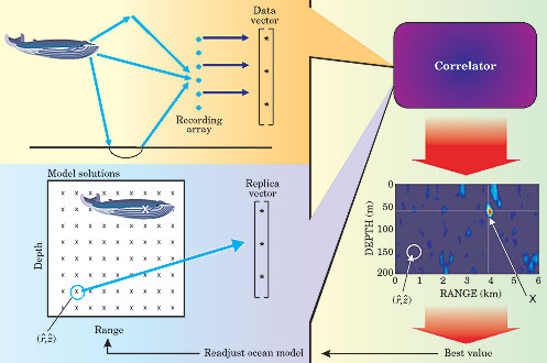
Figure 5. Matched−field processing (MFP). Imagine that a whale sings somewhere in the ocean and you'd like to know where. If your model of waveguide propagation in the ocean is sufficiently reliable, then comparing the recorded soundsthe whale's data vectorone frequency at a time, for example, with replica data based on best guesses of the location (r, z) that the model provides, will eventually find it. The red peak in the data indicates the location of highest correlation. The small, circled x represents a bad guess, which thus doesn't compare well with the measured data. The feedback loop suggests a way to optimize the model: By fine−tuning the focusthe peak resolution in the plotone can readjust the model's bases (the sound−speed profile, say). That feedback describes a signal−processing version of adaptive optics. (Data from ref. 16.)
Box 3. Internal Waves Because of the density stratification of the water column, the coastal oceans support a variety of waves in their interior.17 One particularly important type of wave is the internal gravity wave (IW), a small, horizontal−scale disturbance produced by (among other mechanisms) tidal currents flowing over a sloping sea floor. Two flavors of IWs are found in stratified coastal waters. Linear waves, found virtually everywhere, obey a standard wave equation for the displacement of the surfaces of constant density. Nonlinear IWs, generated under somewhat more specialized circumstances, obey some member of a class of nonlinear equations, the most well known being the Korteweg−de Vries equation. Both types of IWs can be nicely illustrated by a simple two−layer model, like the standard "oil−on−water" toy. Shown here are actual temperature sensor data from a typical coastal−wave system off the south coast of Martha's Vineyard, Massachusetts, on 7 and 8 July 1996.18 The dramatic high−frequency fluctuations in temperature between water layers display the characteristics of a nonlinear internal wave train. Coined a solibore, the wave train is a combination 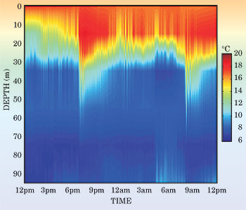 of an internal tidal borethe jump in the thermocline at the onset of the wave trainand solitons, the high−frequency spikes at the boundary of the layers. That is, the IWs exhibit both wave and bore properties. The 6pm and 9am data points, for instance, indicate a dramatic change in the vertical profile of temperature in the ocean. The sharpness of the leading−wave spikes, a measure of the horizontal temperature (or sound speed) gradient, is especially important to acoustics because the horizontal coupling of acoustic normal modes along a propagation track is roughly proportional to that gradient. The nonlinear IWs in shallow water display the strongest gradients of any ocean object except a water−mass front. These nonlinear wave trains also can duct acoustic energy between the solitons (figure 4 shows a schematic), an effect that Mohsen Badiey from the University of Delaware and his collaborators have recently shown.6
|
|
Company Spotlight | ||||||||||||||||
|
|
||||||||||||||||||